Dynamic image reconstruction
Dynamic imaging involves reconstruction of a series of static images across the whole duration of the acquisition time (usually not less than one hour) by dividing the time into usually non-overlapping dynamic time frames. It is assumed that the average tracer concentration during any frame is representative of the whole frame and any concentration changes within the frame are considered minor relative to the changes across the whole acquisition.
Dynamic reconstruction of the Biograph mMR data uses the same function, nipet.mmrchain as shown in section Static image reconstruction for the mMR chain processing. In addition to the basic parameters used, additional parameters need to be defined for dynamic reconstruction.
Dynamic time frame definitions
The extra parameters include the definition of the dynamic time frames. For example, for identical acquisitions, as the provided amyloid PET data (see Raw brain PET data), the one-hour dynamic PET data was divided into 31 dynamic frames in [8], i.e.: 4 × 15s, 8 × 30s, 9 × 60s, 2 × 180s, 8 × 300s, which makes the total of 3600s (one hour).
These definitions can then be represented using Python lists in three ways:
the simplest way—a 1-D list, with elements representing the consecutive frame durations in seconds, i.e., for the above definitions it will be:
frmdef_1D = [
   15,  15,  15,  15,
   30,  30,  30,  30,
   30,  30,  30,  30,
   60,  60,  60,
   60,  60,  60,
   60,  60,  60,
   180, 180,
   300, 300, 300, 300,
   300, 300, 300, 300
   ]
a more elegant representation is by using a 2-D Python list, starting with a string ‘def’, followed by two-element sub-lists with the repetition number and the duration in seconds [s], respectively, i.e.:
frmdef_2D = ['def', [4, 15], [8, 30], [9, 60], [2, 180], [8, 300]]and the last most flexible representation is by using again a 2-D list, starting with a string ‘timings’ or ‘fluid’, followed by two-element sub-lists with the start time, \(t_0\) and the end time \(t_1\) for each frame, i.e.:
frmdef_t = [
         'timings',
         [0, 15],
         [15, 30],
         [30, 45],
         [45, 60],
         [60, 90],
         [90, 120],
         [120, 150],
         [150, 180],
         [180, 210],
         [210, 240],
         [240, 270],
         [270, 300],
         [300, 360],
         [360, 420],
         [420, 480],
         [480, 540],
         [540, 600],
         [600, 660],
         [660, 720],
         [720, 780],
         [780, 840],
         [840, 1020],
         [1020, 1200],
         [1200, 1500],
         [1500, 1800],
         [1800, 2100],
         [2100, 2400],
         [2400, 2700],
         [2700, 3000],
         [3000, 3300],
         [3300, 3600]
         ]
The last representation is the most flexible as it allows the time frames to be defined independent of each other. This is especially useful when defining overlapping time frames or frames which are not necessarily consecutive time-wise.
All the definitions can be summarised in one dictionary using the above frmdef_1D or frmdef_2D definitions, i.e.:
# import the NiftyPET sub-package if it is not loaded yet
from niftypet import nipet

# frame dictionary
frmdct = nipet.dynamic_timings(frmdef_1D)
or
# frame dictionary
frmdct = nipet.dynamic_timings(frmdef_2D)
resulting in:
In [1]: frmdct
Out[1]:
{'frames': array([ 15,  15,  15,  15,  30,  30,  30,  30,  30,  30,  30,  30,  60,
         60,  60,  60,  60,  60,  60,  60,  60, 180, 180, 300, 300, 300,
        300, 300, 300, 300, 300], dtype=uint16),
 'timings': ['timings',
  [0, 15],
  [15, 30],
  [30, 45],
  [45, 60],
  [60, 90],
  [90, 120],
  [120, 150],
  [150, 180],
  [180, 210],
  [210, 240],
  [240, 270],
  [270, 300],
  [300, 360],
  [360, 420],
  [420, 480],
  [480, 540],
  [540, 600],
  [600, 660],
  [660, 720],
  [720, 780],
  [780, 840],
  [840, 1020],
  [1020, 1200],
  [1200, 1500],
  [1500, 1800],
  [1800, 2100],
  [2100, 2400],
  [2400, 2700],
  [2700, 3000],
  [3000, 3300],
  [3300, 3600]],
 'total': 3600}
Please note, that internally, consecutive dynamic frames are represented as an array of unsigned 16-bit integers.
Dynamic reconstruction
The dynamic reconstruction can be invoked after the following setting-up and pre-processing:
import os
import logging
from niftypet import nipet
from niftypet import nimpa

logging.basicConfig(level=logging.INFO)
# dynamic frames for kinetic analysis
frmdef = ['def', [4, 15], [8, 30], [9, 60], [2, 180], [8, 300]]

# get all the constants and LUTs
mMRpars = nipet.get_mmrparams()

#------------------------------------------------------
# GET THE INPUT
folderin = '/path/to/amyloid_brain'

# recognise the input data as much as possible
datain = nipet.classify_input(folderin, mMRpars)
#------------------------------------------------------

# switch on verbose mode
logging.getLogger().setLevel(logging.DEBUG)

# output path
opth = os.path.join( datain['corepath'], 'output')

#------------------------------------------------------
# GET THE MU-MAPS
muhdct = nipet.hdw_mumap(datain, [1,2,4], mMRpars, outpath=opth, use_stored=True)

# UTE-based object mu-map
muodct = nipet.obj_mumap(datain, mMRpars, outpath=opth, store=True)
#-----------------------------------------------------
Since multiple image frames are reconstructed, the mmrchain function apart from 4-D NIfTI image storing, also enables to store intermediate 3-D NIfTI images for each dynamic frame using the option store_img_intrmd = True:
recon = nipet.mmrchain(
         datain,
         mMRpars,
         frames = frmdef,
         mu_h = muhdct,
         mu_o = muodct,
         itr = 4,
         fwhm = 0.,
         outpath = opth,
         fcomment = '_dyn',
         store_img = True,
         store_img_intrmd = True)
The path to the reconstructed 4-D image can be accessed through the output dictionary, recon:
In [2]: recon['im'].shape
Out[2]: (31, 127, 344, 344)
or the stored 4-D NIfTI image in:
In [19]: recon['fpet']
Out[19]: '/path/to/NIfTI-output'
Time offset due to injection delay
In most cases the injection is performed with some delay relative to the time of starting the scan. Also, the first recorded counts will be random events, as the activity is detected from outside the field of view (FOV). The offset caused by the injection delay and random events, can be separated and omitted by running first list mode processing with histogramming, followed by estimating the time offset and accounting for it in the timings of the frames:
# histogram the list mode data (in <datain> dictionary) using scanner parameters (<mMRpars>)
hst = nipet.mmrhist(datain, mMRpars)

# offset for the time from which meaningful events are detected
toff = nipet.lm.get_time_offset(hst)

# dynamic frame timings
frm_timings = nipet.lm.dynamic_timings(frmdef, offset=toff)
The reconstruction is then performed with the augmented timings in the following way:
recon = nipet.mmrchain(
         datain,
         mMRpars,
         frames = frm_timings,
         mu_h = muhdct,
         mu_o = muodct,
         itr = 4,
         fwhm = 0.,
         outpath = opth,
         fcomment = '_dyn',
         store_img = True,
         store_img_intrmd = True)
Note, that the reconstruction pipeline accepts different definitions of the dynamic frames as shown above.
Visualisation of dynamic frame timings
The time frames can be visualised with one line of code:
# draw the frame timings over the head-curve
nipet.lm.draw_frames(hst, frm_timings)
which plots the timings of dynamic frames over the prompts, delayeds and the difference between the two as shown below in Fig. 9.
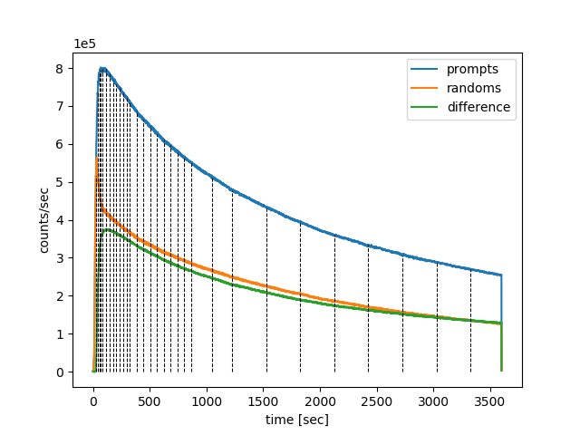
Fig. 9 The dynamic frame intervals are marked with dashed horizontal black curves on top of the head-curve (prompts and delayeds per second).
In order to zoom in to a particular time interval, e.g., from 0s to 150s, and visualise clearly the time offset, the following line of code can be used:
# draw the frame timings over the head-curve, with time limits of tlim
nipet.lm.draw_frames(hst, frm_timings, tlim = [0, 150])
resulting in the following plot (Fig. 10):
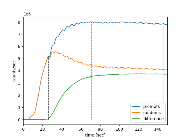
Fig. 10 The dynamic frame intervals are marked with dashed horizontal black curves on top of the part of head-curve (prompts and delayeds per second). Note that almost 30s of list mode data from the beginning is discarded.