Basic PET image reconstruction¶

For basic Siemens Biograph mMR image reconstruction, NiftyPET requires:

PET list-mode data;

component-based normalisation file(s);

the μ-map image (the linear attenuation map as a 3D image).

An example of downloadable raw PET data of amyloid brain scan is provided in Raw brain PET data [1].

Initialisation¶

Prior to dealing with the raw input data, required packages need to be imported and the Siemens Biograph mMR scanner constants and parameters (transaxial and axial lookup tables, LUTs) have to be loaded:

import numpy as np
import sys, os, logging

# NiftyPET image reconstruction package (nipet)
from niftypet import nipet
# NiftyPET image manipulation and analysis (nimpa)
from niftypet import nimpa

logging.basicConfig(level=logging.INFO)
# get all the scanner parameters
mMRpars = nipet.get_mmrparams()

Sorting and classification of input data¶

All the part of the input data is aimed to be automatically recognised and sorted in Python dictionary. This can be obtained by providing a path to the folder containing the unzipped file of the freely provided raw PET data in Raw brain PET data. The data is then automatically explored and sorted in the output dictionary datain:

# Enter the path to the input data folder
folderin = '/path/to/input/data/folder/'

# automatically categorise the input data
datain = nipet.classify_input(folderin, mMRpars)

The output of datain for the above PET data should be as follows:

In [5]: datain
Out[5]:
{'#mumapDCM': 192,
 'corepath': '/data/amyloid_brain',
 'lm_bf': '/data/amyloid_brain/LM/17598013_1946_20150604155500.000000.bf',
 'lm_dcm': '/data/amyloid_brain/LM/17598013_1946_20150604155500.000000.dcm',
 'mumapDCM': '/data/amyloid_brain/umap',
 'nrm_bf': '/data/amyloid_brain/norm/17598013_1946_20150604082431.000000.bf',
 'nrm_dcm': '/data/amyloid_brain/norm/17598013_1946_20150604082431.000000.dcm'}

The parts of the recognised and categorised input data include:

Type	Path
`corepath`	the core path of the input folder
`#mumapDCM`	the number of DICOM files for the μ-map, usually 192
`mumapDCM`	path to the MR-based DICOM μ-map
`lm_bf`	path to the list-mode binary file
`lm_dcm`	the path to the DICOM header of the list-mode binary file
`nrm_bf`	path to the binary file for component based normalisation
`nrm_dcm`	path to the DICOM header for the normalisation

Note

The raw mMR PET data can also be represented by a single *.ima DICOM file instead of the *.dcm and *.bf pairs for list-mode and normalisation data, which will be reflected in datain.

Specifying output folder¶

The path to the output folder where the products of NiftyPET go, as well as the verbose mode can be specified as follows:

# output path
opth = os.path.join( datain['corepath'], 'output')

# switch on verbose mode
logging.getLogger().setLevel(logging.DEBUG)

With the setting as above, the output folder output will be created within the input data folder.

Obtaining the hardware and object μ-maps¶

Since MR cannot image the scanner hardware, i.e., the patient table, head and neck coils, etc., the high resolution CT-based mu-maps are provided by the scanner manufacturer. These then have to be appropriately resampled to the table and coils position as used in any given imaging setting. The hardware and object μ-maps are obtained as follow:

# obtain the hardware mu-map (the bed and the head&neck coil)
muhdct = nipet.hdw_mumap(datain, [1,2,4], mMRpars, outpath=opth, use_stored=True)

# obtain the MR-based human mu-map
muodct = nipet.obj_mumap(datain, mMRpars, outpath=opth, store=True)

The argument [1,2,4] for Obtaining the hardware μ-map correspond to the hardware bits used in imaging, i.e.:

Head and neck lower coil

Head and neck upper coil

Spine coil

Table

Currently, the different parts have to be entered manually (they are not automatically recognised which are in use).

The option use_stored=True allows to reuse the already created hardware μ-map, without recalculating it (the resampling can take more than a minute).

Both output dictionaries muhdct and muodct will contain images among other parameters, such as the image affine matrix and image file paths.

In order to check if both μ-maps were properly loaded, the maps can be plotted together transaxially by choosing the axial index iz along the \(z\)-axis, as follows:

# axial index
iz = 60

# plot image with a colour bar
matshow(muhdct['im'][iz,:,:] + muodct['im'][iz,:,:], cmap='bone')
colorbar()

This will produce the following image:

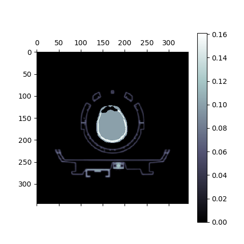
Fig. 2 Composite of the hardware and object μ-maps. Observed can be the human head between the upper and lower head&neck coils, and the patient table below.

The sagittal image can be generated in a similar way, but choosing the slice along the \(x\)-axis, i.e.:

# axial index
ix = 170

# plot image with a colour bar
matshow(muhdct['im'][:,:,ix] + muodct['im'][:,:,ix], cmap='bone')
colorbar()

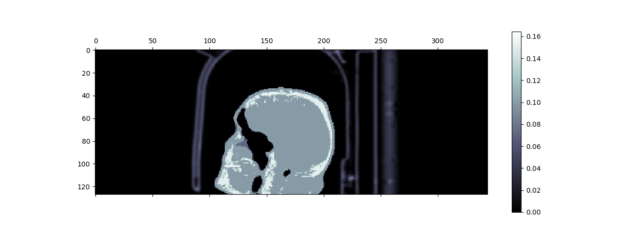
Fig. 3 Sagittal view of the composite of the hardware and object μ-maps. Observed can be the human head between the upper and lower head&neck coils, and the patient table on the right of the head.

List-mode processing with histogramming¶

The large list-mode is processed to obtain histogrammed data (sinograms) as well as other statistics on the acquisition, including the head curves and motion detection:

hst = nipet.mmrhist(datain, mMRpars)

The direct prompt and delayed sinograms can be viewed by choosing the sinogram index below 127 and from 127 up to 836 for oblique sinograms, i.e.:

# sinogram index (<127 for direct sinograms, >=127 for oblique sinograms)
si = 60

# prompt sinogram
matshow(hst['psino'][si,:,:], cmap='inferno')
colorbar()
xlabel('bins')
ylabel('angles')

# delayed sinogram
matshow(hst['dsino'][si,:,:], cmap='inferno')
colorbar()
xlabel('bins')
ylabel('angles')

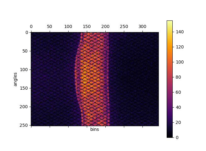
Fig. 4 Direct prompt sinogram for 60 minute amyloid PET acquisition.

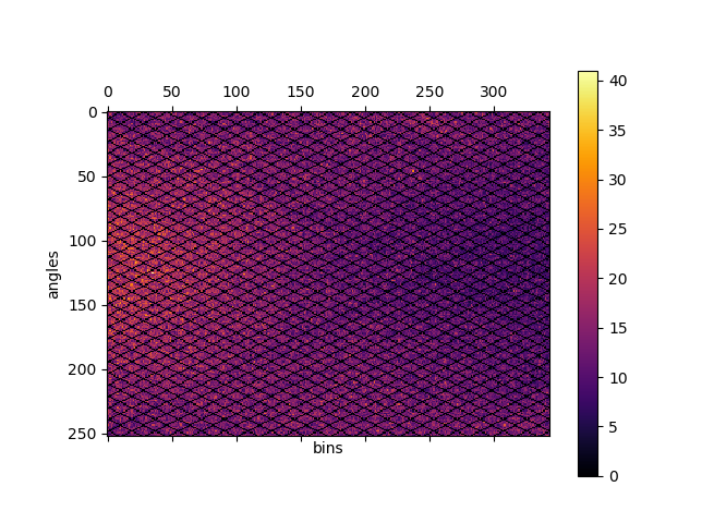
Fig. 5 Direct delayed sinogram for 60 minute PET acquisition.

The head-curve, which is the total number of counts detected per second across the acquisition time, for the prompt and delayed data can be plotted as follows:

plot(hst['phc'], label='prompt')
plot(hst['dhc'], label='delayed')
legend()
grid('on')
xlabel('time')
ylabel('counts')

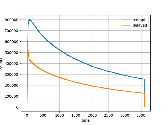
Fig. 6 Head curve for prompt and delayed events for the 60-minute acquisition.

In order to get general idea about the potential motion during the acquisition, the centre of mass of the radiodistribution along the axial direction can be plotted as follows:

plot(hst['cmass'])
grid('on')
xlabel('time')
ylabel('Centre of mas of radiodistribution')

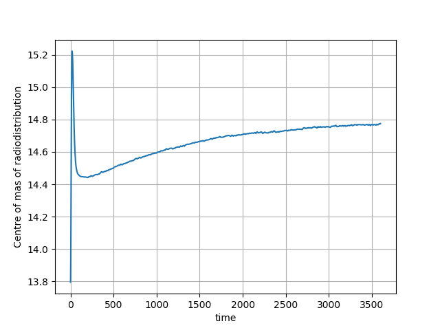
Fig. 7 The centre of mass of the radiodistribution for the 60-minute amyloid PET acquisition. Very little motion is observer–the smooth, exponentially varying curve is due to the tracer kinetics.

Static image reconstruction¶

The code below provides full image reconstruction for the last 10 minutes of the acquisition to get an estimate of the amyloid load through the ratio image (SUVr).

recon = nipet.mmrchain(
    datain, mMRpars,
    frames = ['timings', [3000, 3600]],
    mu_h = muhdct,
    mu_o = muodct,
    itr=4,
    fwhm=0.0,
    outpath = opth,
    fcomment = 'niftypet-recon',
    store_img = True)

The input arguments are as follows:

argument	description
`datain`	input data (list-mode, normalisation and the μ-map)
`mMRpars`	scanner parameters (scanner constants and LUTs)
`frames`	definitions of time frame(s);
`mu_h`	hardware μ-map
`mu_o`	object μ-map
`itr`	number of iterations of OSEM (14 subsets).
`fwhm`	full width at half-maximum for the image post-smoothing
`outpath`	path to the output folder
`fcomment`	prefix for all the generated output files
`store_img`	store images (yes/no)

the argument timings indicates that the start/stop times in the following sublist is user-specified and can be done for multiple time frames (see section Dynamic time frame definitions).

The reconstructed image can be viewed as follow:

matshow(recon['im'][60,:,:], cmap='magma')
colorbar()

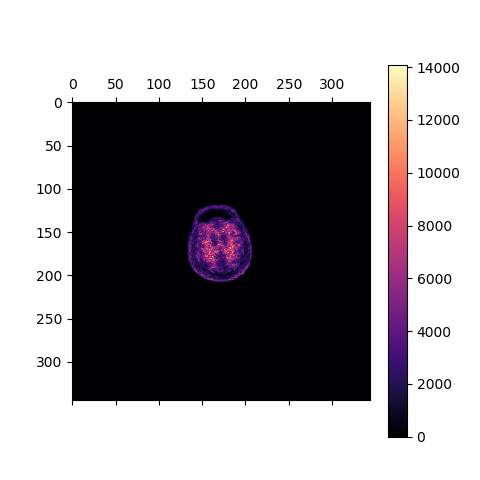
Fig. 8 The transaxial slice of the amyloid PET reconstructed image. Voxel intensities are in Bq.